Photoelectric Effect Simulator App
Background:
The photoelectric effect was one of the earliest experimental observations to demonstrate the quantization of light. First documented in 1887 by Heinrich Hertz, the effect describes the phenomenon of electrons being liberated from a metal placed in the path of a beam of sufficiently energetic monochromatic light. Along with blackbody radiation, the classically inexplicable observations resulting from the photoelectric effect were among the earliest evidence to support the argument for the quantization of light, which Albert Einstein employed in 1905 to explain the effect mathematically.
The experiment is typically set up with a small plate of the material being tested for its photoelectric properties connected to the positive terminal of a variable voltage supply, in which configuration it is called a photocathode. A negatively charged opposing anode plate is then positioned such that it is shielded from the incoming light, and connected to the negative end of the voltage supply, and both plates are encased in a vacuum tube to isolate them from contamination. This device is known as a photocell. Although the orientation of the voltage supply causes the electrons within the photocathode to face an electric tension that holds them within that plate, the anode attracts electrons that achieve sufficient energy from the incident radiation to break free from the photocathode, completing the circuit and causing a measurable flow of current while potential remains below a certain threshold, or stopping voltage . To measure the current caused by these liberated photoelectrons, a highly sensitive microammeter is placed in series with the photocathode, while a voltmeter is placed in parallel with the photocell.
In an ideal system, when increasing the opposing voltage at the supply for a fixed frequency of incident radiation, the flow of current attributable to these photoelectrons decreases until no electrons have sufficient kinetic energy to break free of the potential and current stops flowing, at what is referred to as the stopping voltage. This voltage represents the maximum kinetic energy of the photoelectrons, before the potential exceeds the energy available for photoelectrons to become liberated from the surface.
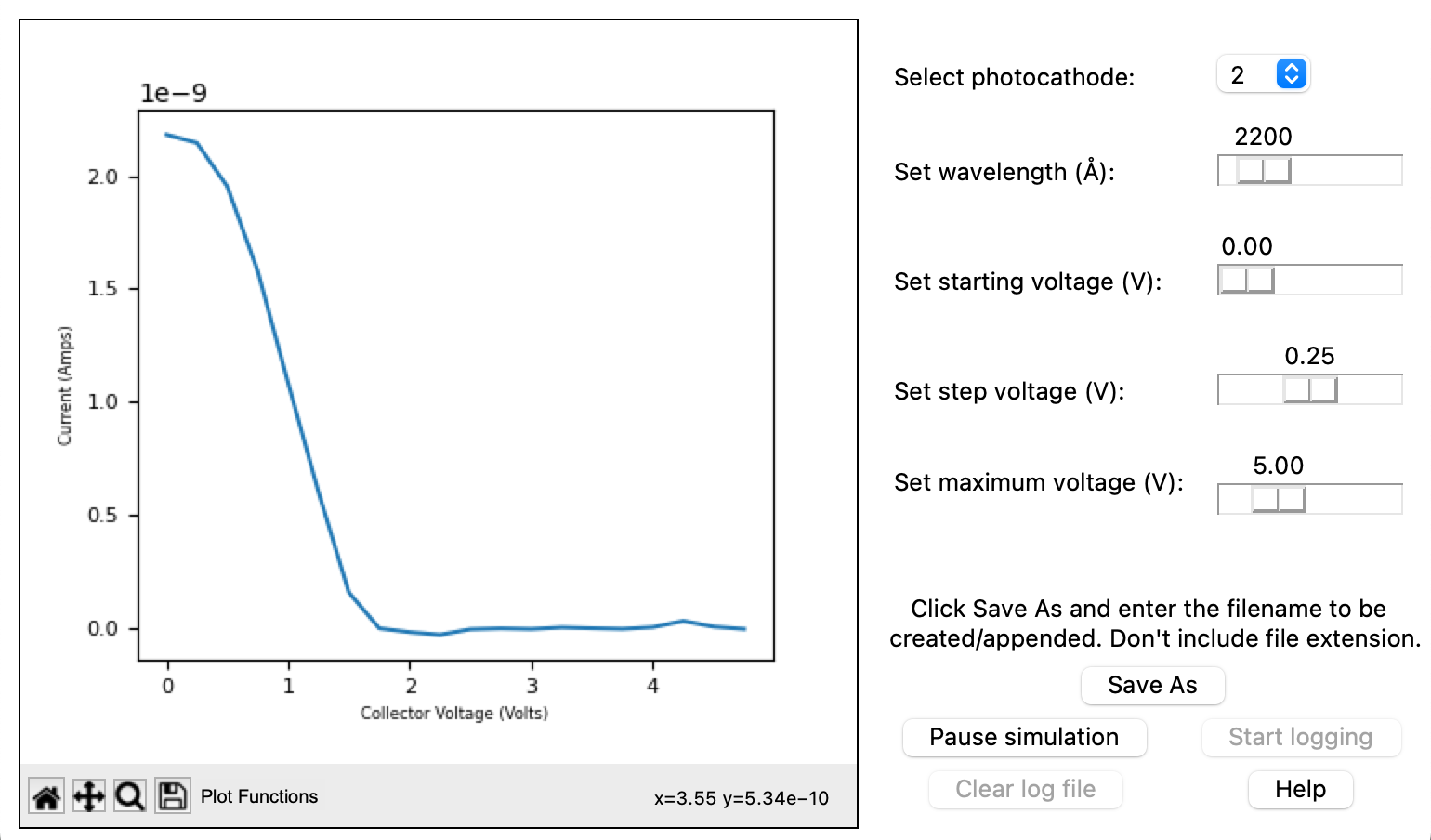
This program uses a model of the photoelectric effect to allow users to select from a predefined list of six photocathode materials, and to define incident light wavelength, voltage range and step size in a compact graphical user interface. The program then uses these data to create a graph of voltage vs photocurrent using the matplotlib Python library. The GUI is written using the Python Tkinter library that comes as part of the standard Python distribution, and generates an output CSV log file with basic controls from within the application using the standard Python csv library. The program also detects some common, forseeable user errors, and ensures input parameters are suitable for calculations before proceeding.
Setting up the GUI:
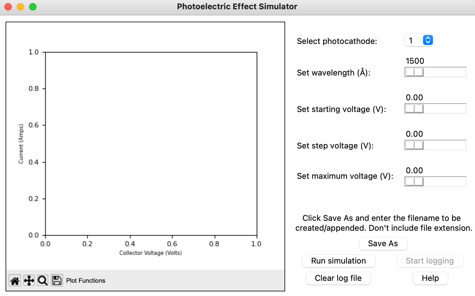
The program is built around the Tkinter library, which uses frames transposed on a main window to organize the GUI. The first step taken in building the working application was to configure a main window with the necessary user inputs, which would later be mapped to the applicable functions. The program is designed to take user inputs for wavelength of the incident light, starting voltage, voltage step size, and maximum voltage, and allows the user to select from one of six unnamed photocathode materials. The user can also specify a log file to write data to in a comma seperated value format, if they so choose.
The program used the following libraries, which will be explained in further detail as they are used.
from tkinter import *
from tkinter import filedialog
from matplotlib.figure import Figure
from matplotlib.backends.backend_tkagg import (FigureCanvasTkAgg, NavigationToolbar2Tk)


import numpy as np
import random as r

import csv, time, threading
The main Tkinter window was initialized by defining the size in pixels, the background color, and the window name, and defining a variable for the main window, to be referenced when creating frames. Tk() is Tkinter's method for creating a new window. All code that exists within the window must be inside window.mainloop(), which keeps the Tkinter window active. These are the most basic aspects of all Tkinter programs, and on their own, would simply create a blank, white, 770 x 460 px window with the name "Photoelectric Effect Simulator."
# Intializing the tkinter window

window = Tk()
window.title("Photoelectric Effect Simulator")
window.geometry("770x460")
window.configure(bg = "White")

window.mainloop()
This window was subdivided into three frames, although more or fewer could have been used, depending on how the window layout was planned. plotFrame holds the plot, and is surrounded with a black border using the highlightbackground option of Frame(). While initially positioning the other frames, borders were added as well to determine their boundaries, but were later removed for asthetic purposes. Note that in each Frame(), the first argument is the window that the frame sits in. Tkinter supports multiple methods of positioning objects in a window, ranging from defining positions in a pixel-by-pixel coordinate system to positioning objects relative only to one another. A useful compromise between these options is the .grid() method, which automatically subdivides the space containing the object for which the method is being called based on the total number of rows and columns defined for all objects in that space. As an example, all three frames shown below are children of the main window, and a total of two columns and two rows are defined (the largest value of both row and column is 1). The position of each Frame() can therefore be specified by a row and column coordinate in that grid. By using options rowspan and columnspan, an object can be assigned to occupy multiple rows or columns in a grid. padx and pady are used to define padding from the edge of the frame and from other objects in the x and y directions in pixels.
# Frames

plotFrame = Frame(window, highlightbackground = "black", highlightthickness=1)
guidedParamFrame = Frame(window, bg="white")
simControlsFrame = Frame(window, bg="white")

# Frame positions

plotFrame.grid(rowspan=2, column=0, padx = 10, pady = 10)
guidedParamFrame.grid(row = 0, column= 1)
simControlsFrame.grid(row = 1, column = 1)
Next, user inputs were created in the frames. The major widgets used within the frames are Label(), which creates a text field, OptionMenu(), which creates a dropdown selection menu, Scale(), which creates a slider, and Button(). Each of these widgets is positioned using the .grid() method, with the first argument being the frame that they occupy. Some of these widgets also use the ipadx and ipady options in their positioning, which allows for the addition of internal padding for the widget, e.g. making a button wider by adding space on either side of the button text. Objects can also be anchored to a certain side of their grid position using the sticky option and defining the cardinal directions of the desired position. For example, to place a widget in the top left corner, sticky = "NW" can be used. Examples of the photocathode material selection dropdown and label, and the wavelength slider and label are shown below. The * preceding the range() argument of OptionMenu allows the elements of the list to be unpacked and passed individually. For example, if the list produced by range(1, len(photocathodeMaterials)+1) consists of values (1,2,3), passing *range(1, len(photocathodeMaterials)+1) is equivalent to passing 1, 2, 3 to the function manually. This is also called unrolling the list. All the sliders, as well as the photocathode dropdown are grouped in guidedParamFrame.
# Photocathode dropdown
photocathodeLabel = Label(guidedParamFrame, text= "Select photocathode:", bg="white")
photocathodeLabel.grid(row=0, column=0, sticky="W", padx = 3)
clicked = IntVar(value=1)
photocathodeComboBox = OptionMenu(guidedParamFrame, clicked, *range(1, len(photocathodeMaterials)+1)) # These values are indices of true photocathode material workfunctions, defined in photocathodeMaterials.
photocathodeComboBox.config(bg = "white")
photocathodeComboBox.grid(row=0, column=1, padx=10, sticky = "W", ipady =10)

# Wavelength slider
wavelengthLabel = Label(guidedParamFrame, text="Set wavelength (Å):", bg="white")
wavelengthLabel.grid(row=1, column = 0, sticky="W", padx = 3)
wavelengthSlider = Scale(guidedParamFrame, bg = "white", troughcolor="white", showvalue=True, from_ = 1500, to = 7000, orient="horizontal")
wavelengthSlider.grid(row = 1, column = 1, ipady = 10, padx =10)
Controls for the logging portion of the program are separated into simControlsFrame, and use the format shown below. Each button is connected to a callback–or a function called by another function–that accepts no arguments, and will be invoked at each button press.
# File name prompt field
filePrompt = Label(simControlsFrame, text="Click Save As and enter the filename to be \n created/appended. Don't include file extension.", bg = "white")
filePrompt.grid(row = 0, column =0, columnspan=2)
fileSave = Button(simControlsFrame, text = "Save As", highlightbackground= "white", command = fileOpen)
fileSave.grid(row = 1, column = 0, columnspan = 2)
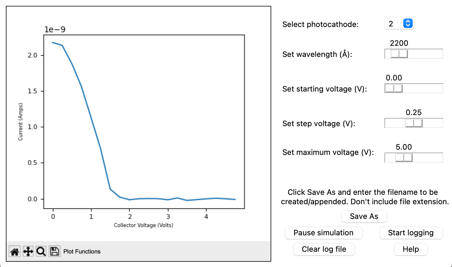
The logging button recieves special treatment, as it is not possible to log data when data is not being collected. As such, the ["state"] of the button is set equal to "normal" or "disabled" as follows, and is manipulated according to whether the conditions for logging are satisfied. When the button is "disabled", it remains visible, but is grayed out and not clickable.
# Start/stop logging button
log = Button(simControlsFrame, text="Start logging", highlightbackground="white", command = initiateCSV)
log["state"] = "disabled"
log.grid(row=2, column = 1 )
A help window was also created to walk users through the steps of operating the program, and to provide information about the program and the photoelectric effect generally.
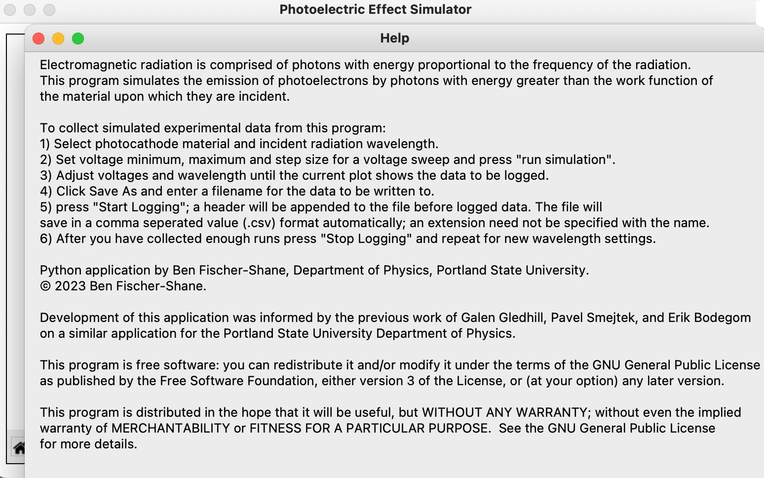
This window is defined using the Tkinter method Toplevel(window), which creates an additional window on top of the original window. While Tkinter will only allow one main window to be created, many toplevel windows can be added. These windows are ideal for adding additional information or functionality outside the scope of the main window. The window is created as shown below, and contains a Label() with the help text.
def openHelpWindow():
    # Toplevel object which will
    # be treated as a new window
    helpWindow = Toplevel(window)

    # sets the title of the
    # Toplevel widget
    helpWindow.title("Help")

    # sets the geometry of toplevel
    helpWindow.geometry("750x450")

    # Label exists here with window text

# Help button
help = Button(simControlsFrame, text="Help", highlightbackground="white", command=openHelpWindow)
help.grid(row=3, column=1)
The clear button for the log file uses a special type of Python function called a lambda function. A lambda function is a nameless one line function that takes the form lambda argument(s): expression. In this case, no arguments are passed to the lambda function, it simply opens the log file stored at filepath in "w" or write mode, which clears the file's contents. This button is also "disabled" at first, until the user defines a file to be stored at filepath.
# Clear log file button
clrLog = Button(simControlsFrame, text = "Clear log file", highlightbackground="white", command = lambda: open(filepath, "w"))
clrLog["state"] = "disabled"
clrLog.grid(row=3, column = 0)
At this point, all the widgets are defined, though the functions that they go to are not, meaning that clicking them will throw an error on the command line (or do nothing, if the command argument is omitted). Next, a plot must be created, functions defined, and mathematical modelling implemented. Finally, the code will be compiled into a standalone app.
Setting up the plot
Matplotlib module backends.backend_tkagg allows for interfacing the very useful matplotlib library with Tkinter. FigureCanvasTkAgg creates a special canvas that can function as a Tkinter widget while also holding matplotlib plots, and NavigationToolbar2Tk creates a toolbar that provides functionality like zooming in on and saving plots.
The setup for the plot looks relatively similar to the use of matplotlib's pyplot module.
# Initializing the plot

fig = Figure(figsize = (4.5, 4))
fig.subplots_adjust(left=0.14, bottom=0.14)

# Adding the subplot and setting blank axes

graph = fig.add_subplot(111)
axisLabels()

# Creating the Tkinter canvas
# Containing the Matplotlib figure
canvas = FigureCanvasTkAgg(fig, master = plotFrame)
canvas.draw()
Some default functionalities that come with the NavigationToolbar2Tk were not needed, so the buttons in the toolbar were customized with the activeToolbar class. This is the only use of classes in this program, which is a point for potential refinement in the future, as object-oriented programming often lends itself to greater concision and readability. Here, the activeToolbar object is defined by class, and takes the NavigationToolbar2Tk function as an argument. The toolitems list takes the format of the original buttons, but only invokes those being used in the program. The __init___ function is a standard part of classes, and is invoked automatically when the class is first instantiated. Here, the super() function is called when the class is first instantiated, and gives access to the methods of the parent class, which is NavigationToolbar2Tk. In this case, it simply creates the toolbar from the parent class when activeToolbar is invoked, with only the toolitems listed. self is always the first argument passed to __init__, and creates a biding to the methods of a class' objects. For example, self.label creates the label widget for each instance of the activeToolbar class.
class activeToolbar(NavigationToolbar2Tk):
    toolitems = (
            ('Home', 'Revert to original view', 'home', 'home'),
            ('Pan', 'Pan view', 'move', 'pan'),
            ('Zoom', 'Zoom', 'zoom_to_rect', 'zoom'),
            ('Save', 'Save plot as image', 'filesave', 'save_figure'),
            )
    def __init__(self, canvas, parent):
        super().__init__(canvas, parent)

        self.label = Label(self, text = "Plot Functions", font=("Arial", 10), bg="gray92")
        self.label.pack(side="left")
The toolbar is placed on the plot pane as follows, and the matplotlib canvas was initialized then positioned using the .pack() method, which places the object relative to other objects. Since this is the only object in this frame, it is somewhat simpler to use pack, although a 1 x 1 grid could easily have been used.
# Instantiating the navigation toolbar
toolbar = activeToolbar(canvas, plotFrame)
toolbar.update()

# Placing the canvas on the Tkinter window
canvas.get_tk_widget().pack()
Setting up the CSV handling
The csv file is opened and configured through three main dedicated functions, shown below. Since the csv will be needed in different parts of the code, the function csvWriter(array) can be called to open the file stored at filepath in "a" (append) mode, and append the argument (a multidimensional list, where each dimension is placed on a new row) to the csv file. newline = "" standardizes the newline escape character, since some systems can try to insert their own newline characters. writerows will append each element of the input list argument to its own line in the csv. For example, [[1,2,3],[4,5,6]] would append two new lines to the csv, the first being 1,2,3 and the second being 4,5,6, with each element separated by a comma.
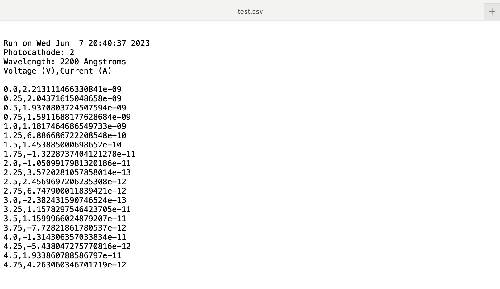
initiateCSV() creates the header for each run, with the photocathode material selected, the wavelength, and column headers for voltage and current values to be appended later. The header also includes the time at which the program was run, which is accessed through the .asctime() method of the time module, which returns the weekday, month, day, and time (in 24 hour format). The .get() method is a property of Tkinter widgets that returns their current value. InitiateCSV only works if the boolean runActive variable, which changes based on whether the run button has been pressed, is set to True. The .config method of Tkinter widgets allows for the options of that widget to be configured or changed later, and in this case is used to change the text on the buttons to prompt users to stop logging if a run is currently active, and vice versa. The global keyword before the logging variable allows any changes to the value stored in logging to be changed across the whole program, since the logging variable is defined for the whole program.
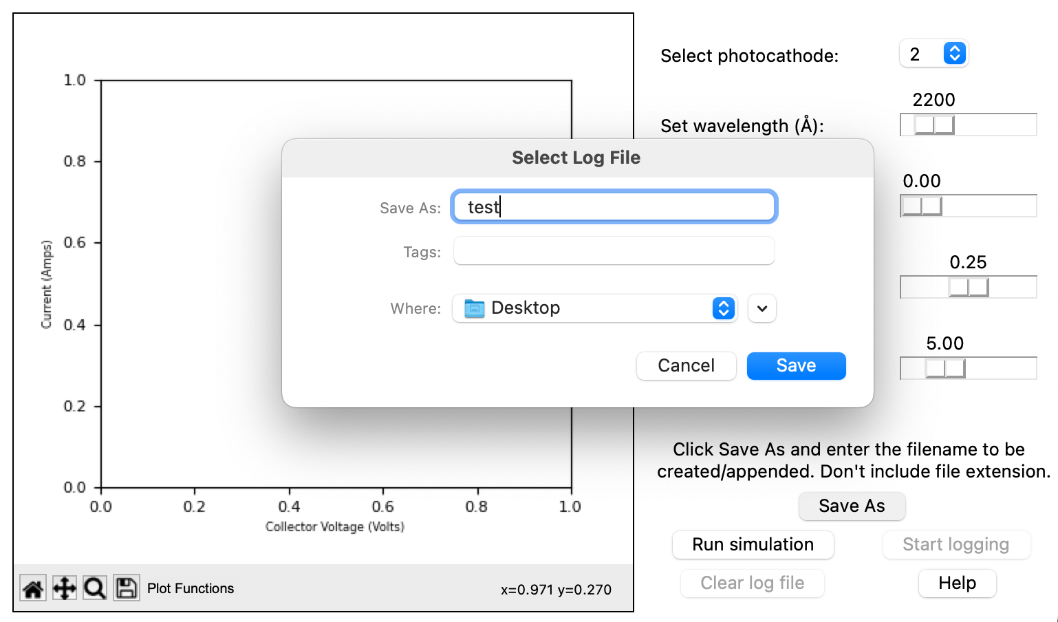
fileOpen() creates the dialog box that pops up to prompt users to enter the name of the file they want to create or append data to. The Tkinter method filedialog.asksaveasfile() creates a default system file save prompt, and the .name method returns the name of the file and its path. The conditional logic that follows checks if the user has entered a filename, and if they have, enables the button to clear the log file, and if data is currently being generated, to append to the newly defined file as well.
def csvWriter(array):
    with open(filepath, "a", newline = "") as output:
        writer = csv.writer(output, delimiter= ",")
        writer.writerows(array)

def initiateCSV():
    global logging
    if runActive == True and logging == False and filepath != "":
        csvWriter([[],
                [],
                [f"Run on {time.asctime(time.localtime(time.time()))}"],
                [f"Photocathode: {clicked.get()}"],
                [f"Wavelength: {wavelengthSlider.get()} Angstroms"],
                ["Voltage (V)", "Current (A)"],
                []]
                )
        log.config(text = "Stop logging", fg = "black")
        logging = True
    elif logging  == True:
        log.config(text = "Start logging", fg = "black")
        logging = False


def fileOpen():
    global filepath
    filepath = filedialog.asksaveasfile(mode = "a", title = "Select Log File", defaultextension=".csv", confirmoverwrite = False).name
    if filepath != "":
        clrLog["state"] = "normal"
        if runActive:
            log["state"] = "normal"
Creating code for running and logging
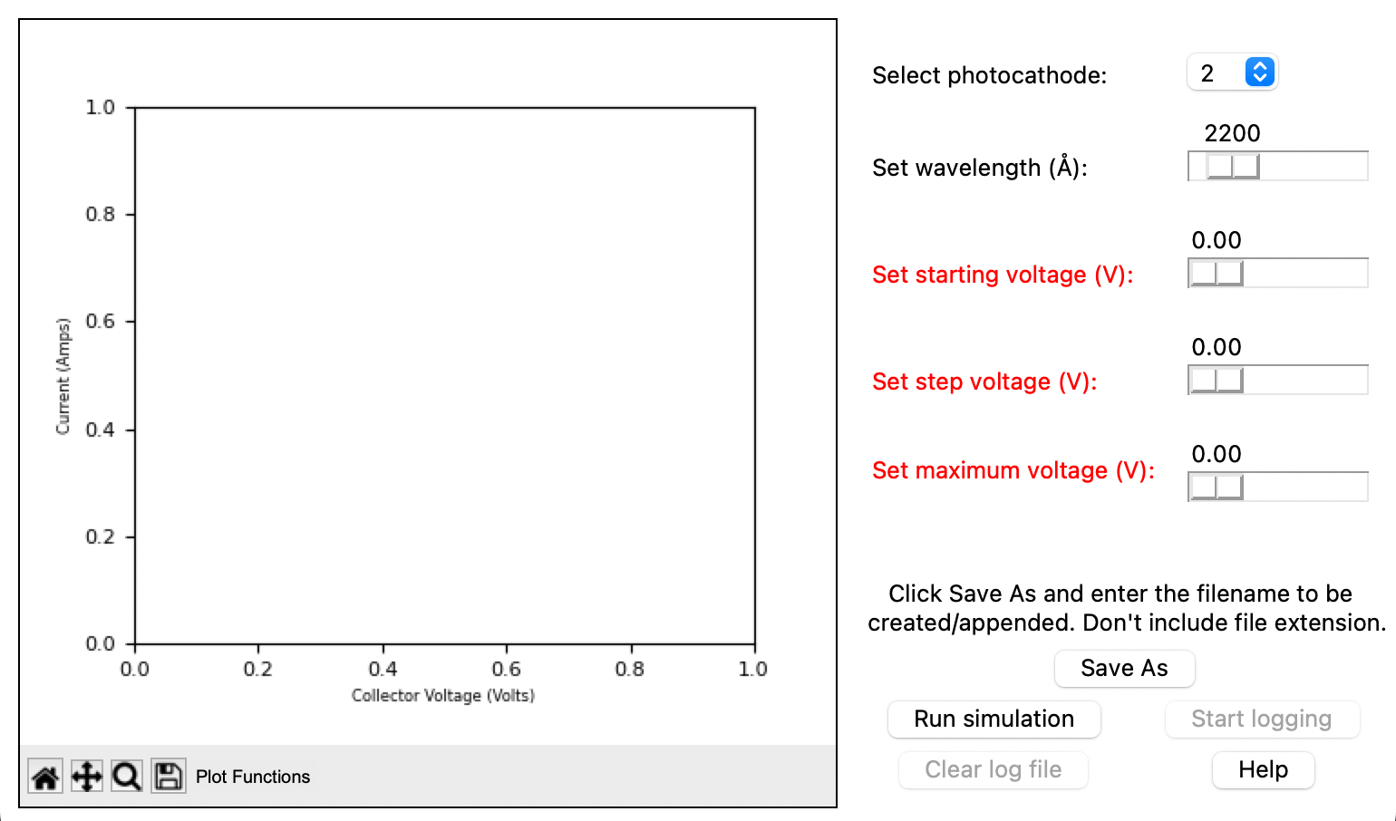
The runSim() function shown below holds the code for running the simulation and logging data. graphLog() contains the code for data handling during an active run and for logging that data, and runs in a while loop as long as run is True. The conditional logic at the start of graphLog() implements a form of error handling, which is somewhat more digestible for long functions than using try/except blocks. The downside of this method is that if an error occurs that is not explicitly accounted for in the conditional logic, the program does not have an error handling scheme to address the error and exit from the problematic code cleanly. For readability and ease of future development, the tradeoff was deemed worthwhile. The exception handling addresses possible issues like a run being initiated while the starting voltage is greater than the stopping voltage.
The mathematics for the program are based on another program written by Galen Gledhill, Pavel Smejtek, and Erik Bodegom for the PSU physics department in 2013, and differs from other programs found online. The equations employ four random variables, and manipulate those values so that noise follows a realistic trend.
A for loop cycles through each x data point in the range between the user-defined starting and stopping voltages, applies the formula, and adds the data points to the output csv if logging is active.
graph.cla clears the graph axes, and all data on the graph.
Implementing threading
Threading allows for multiple processes to run concurrently in a Python application. In this case, a separate thread is used to implement the graphing animation manually, by refreshing the plot data once per second within the graphLog() function. In this way, other parts of the program can continue to function, while the animation creates new values for the plot once per second and uses time.sleep() to create the delay.
def runSim():
    global runActive, run, logging
    # Control the animation

    def graphLog():
        global vDataRange, photonEnergy, workFunction, maxKE, runActive
        while run:
            startVoltage=startVoltageSlider.get()
            maxVoltage = maxVoltageSlider.get()
            stepVoltage = stepVoltageSlider.get()

            if startVoltage >= maxVoltage:
                stepVoltageLabel.config(fg = "black")
                startVoltageLabel.config(fg = "red")
                stVoltageLabel.config(fg = "red")
                if stepVoltage == 0:
                    stepVoltageLabel.config(fg = "red")
                runPause.config(text = "Run simulation")
                log["state"] = "disabled"
                runActive = False
                break
            elif stepVoltage == 0 or stepVoltage > maxVoltage:
                stVoltageLabel.config(fg="black")
                stVoltageLabel.config(fg = "black")
                stepVoltageLabel.config(fg = "red")
                runPause.config(text = "Run simulation")
                log["state"] = "disabled"
                runActive = False
                break

            startVoltageLabel.config(fg="black")
            stVoltageLabel.config(fg = "black")
            stepVoltageLabel.config(fg = "black")

            #The following equations are from a previous photoelectric effect simulator. See credits in "Help" window.
            vDataRange = np.arange(startVoltage, maxVoltage, stepVoltage)
            photonEnergy = (6.626e3 * 2.9979) / (1.602 *wavelengthSlider.get()) # hc/eL in eV
            workFunction = photocathodeMaterials[clicked.get()-1]

            maxKE = photonEnergy - workFunction/1.488
            x0 = photonEnergy/(8.625e-5*6000)
            h0 = x0**2/(np.exp(x0)-1)

            x = vDataRange
            y = []
            for i in range(len(x)):
                voltage = vDataRange[i]
                j3 = 0.0
                r1 = r.random()
                r2 = r.random()
                e4 = (-2*np.log(r1))*(0.5-r2)/np.abs(0.5-r2)
                # ~[-20 ...+20]
                j4 = 5e-12*e4
                if maxKE >0 and voltage <= maxKE:
                    j1 = np.cos(np.pi*voltage/(2*maxKE))
                    r1 = r.random()
                    r2 = r.random()
                    e2 = (-2*0.05*np.log(r1))**2*(0.5-r2)/abs(0.5-r2)
                    j2 = e2*j1
                    j3 = (j1+j2)*h0*1e-6
                y.append(j3+j4)

                if logging:
                    csvWriter([[voltage, y[i]]])
            if logging:
                csvWriter([[],[]])
            graph.cla()
            axisLabels()
            graph.plot(x, y)
            canvas.draw()
            time.sleep(1)

    # If starting a run
    if runActive == False:
            run = True
            threading.Thread(target = graphLog).start()
            if filepath != "":
                log["state"] = "normal"
            runPause.config(text = "Pause simulation")

    else:
        runPause.config(text = "Run simulation")
        log.config(text = "Start logging")
        log["state"] = "disabled"
        logging = False
        run = False

    runActive = not runActive
Compiling into a standalone application
With the code working, the final step to make this code more portable is compiling it into a standalone application. This is done using pyinstaller, which can be installed typing pip install pyinstaller from the command line. The working directory is switched to the same directory that contains the python file, and pyinstaller --onefile --windowed --icon=iconName.icns filename.py is run to compile the code in filename.py into an application, where --onefile bundles the application together into a single file, --windowed compiles without a terminal window for output, and iconName is the desired icon in .icns format, also in the same folder. After running, pyinstaller creates two folders, build and dist. The build folder is not strictly necessary to the operation of the application, and contains metadata that can be used for debugging. The dist folder contains the final application, which can be opened and used as a standalone app!
Conclusion This project brings together many different Python libraries and techniques to create a standalone photoelectric effect application. This app can be used to calculate the workfunctions of the photocathode matierials, and to experimentally determine Planck's constant. It includes some basic exception handling capabilities, and is meant to be an easy-to-use introductory tool that abstracts the somewhat more obscure math behind its processes. The application can be found on my GitHub here, so feel free to try it yourself and let me know what you think!